
How to make spatial locality work for you: the tiles concept

How do you run a machine learning model over an entire state without blowing up in memory or runtime? At Mach9, we often have a need to run a piece of code over a very large geographic or spatial dataset. For example, we have a ML model that takes in a point cloud and imagery of an area and locates all of the relevant curb-related lines.
However, as we scale up the area of our inputs to our code, often times our code’s runtime or memory usage scales superlinearly. For example, as the size of an image doubles in length, or as its resolution doubles, the number of pixels quadruples.
As a concrete example, let’s say that you’re working with a top-down view of an area at 2cm resolution. Then a 10m by 10m area would have 250,000 pixels. But at 1cm resolution, that same area would have 1,000,000 pixels - a 4x increase. And a 100m by 100m area would have 25,000,000 pixels, probably too much for any model to take in as a single unit.
Luckily, we have a property that we can exploit for our typical pieces of code for spatial analysis - they’re local. What this means is that
Their outputs are spatially organized, and
their outputs only depend on regions of the input “near” to them.
In other words, the output of your code at a location x only depends on points “close by” to x, let’s say within ε meters. (For the non-math nerds, that letter is called epsilon, and it typically represents a small number.) Think of ε as a “horizon of relevance” - how far away your algorithm needs to look in order to make a decision. At Mach9, we call ε the “bleed”, for reasons we’ll see below.
Many real-world things have this locality property, especially when it comes to surveying. The position of a manhole in one part of a roadway isn’t really influenced by the position of other objects far away - in theory, you should be able to locate a manhole in an area given only the point cloud and images near that manhole, without looking like a mile away. For manholes, for example, ε might be a couple of meters - beyond a couple of meters away from the center of the manhole, the points don’t really matter.
When you want to run a local function on a large area, you can use what we call tiles to make your code more efficient. Here’s the recipe:
Define some tiling scheme over the area that you want to run your code or function on. The tiling scheme is a set of regions, all of which cover the area.
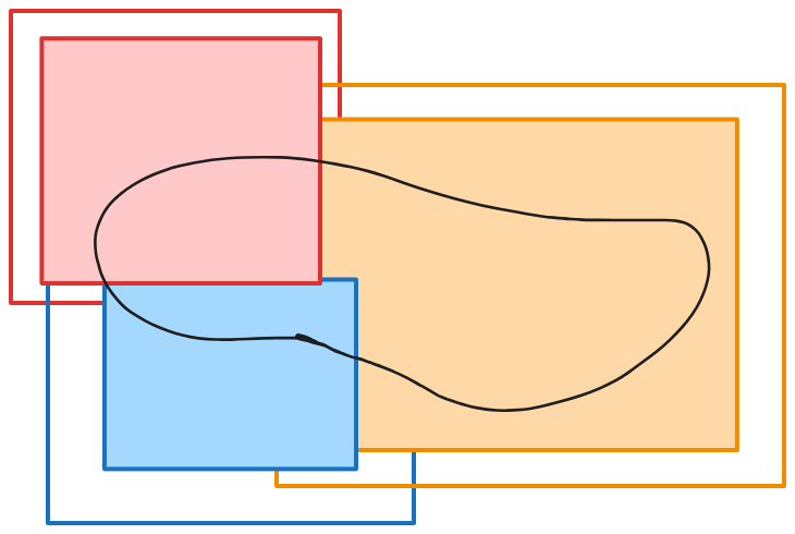
Your tiling scheme needs to be covering in an overlapping way. In particular, every point in your area of interest needs to be at least ε meters away from the boundary of some tile. In other words, for any point, you can draw a circle or ball of radius ε around it, and the entire circle or ball would be part of at least one single tile. Overlap is OK here - your ball can be entirely contained within many different tiles, and so can your point.

A tiling scheme over a region in black - notice how the tiles overlap significantly. Red, blue, and orange are the tiles in the tiling scheme. The green circle around the edge of the region is entirely contained inside the orange tile. One way of creating this overlap-by-ε condition is to generate tiles that are exactly adjacent, or overlap a little, and expand them all by ε in all directions. That’s why we call this the bleed - we’re basically bleeding over each tile a bit in each direction.
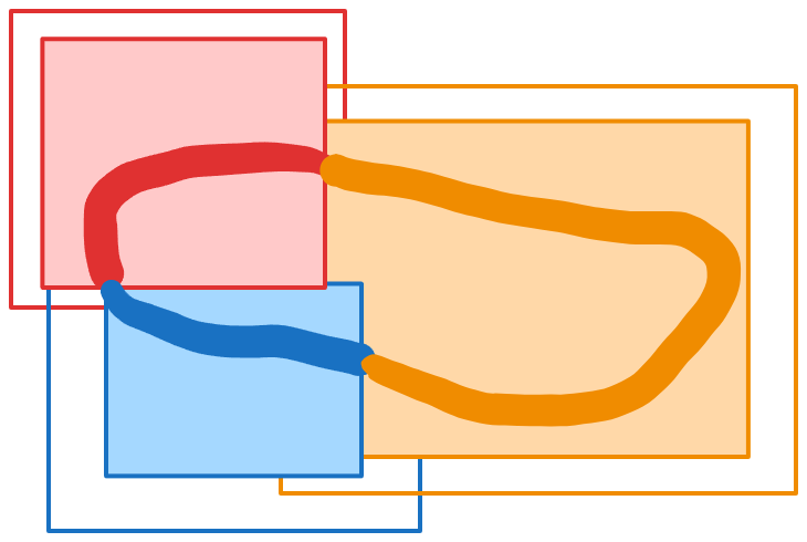
Run your code on each tile separately. You can do this totally in parallel - this is how Mach9 processes very large datasets quickly.
Now combine your results. Since your output is spatially defined, we need to define an output to put for every point in space. This can be accomplished in two ways:
For every point, follow these steps:
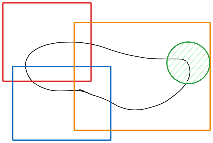
Pick some tile so that a circle or ball around the point of radius ε is entirely contained within that tile. The covering property from step 1 guarantees that at least some such tile exists.
Because of the locality property of your code, it doesn’t matter which tile you pick! All tiles with enough border around the point will agree at the point. Therefore, you can just pick whatever tile you want to copy your output from.
If you don’t want to do something for every single (uncountably many) point of R^3, you can also do this tile-picking en masse:
For each tile, define its interior - the set of all points that are at least ε meters away from the edge of the tile. If you created your tiles with a bleed from step 1, you can just use the original, non-bled tiles.
Partition your entire space into non-overlapping but completely covering interiors by cutting away some interiors. Like above, it doesn’t matter which tile interior you pick for any part of your space - all tile interiors will agree when they overlap.
The interiors of the tiles; they’ve been cropped so that they don’t overlap Crop each tile’s output to the non-overlapping interior set defined above.
Areas of the region assigned to each tile. Notice that at the boundaries of the different assignments, the region matches up. Put all tile outputs in the same space, and connect up any seams at the edges. For example, if you’ve cropped a line at an interior boundary, the locality property guarantees that the two ends of the line across the boundary will exactly match.


Example: machine learning
Let’s say that you’re running an object detector on a very large image, 10,000 by 10,000 pixels. Typical vision transformers will have a VRAM usage that scales quadratically with the pixel width of the image, so this seems like a big no-no. However, if our image is very large relative to the size of the object we’re detecting, we can use tiles to break it up. For example, if our objects are typically around 100 pixels in size, we can set the bleed to be 200 pixels or so, split up our 10,000 by 10,000 pixel image into much more manageable 2000 by 2000 pixel chunks, run the model on each one, and combine the detection results at the end. Where our chunks overlap, the model should agree, so combining will be easy. This lets you cut your VRAM usage by 75% while still maintaining your result accuracy.
Example: task splitting
At Mach9, we offer the ability to split up your 50 mile datasets into a set of tasks so that you can have multiple drafters working on the same dataset. How do we make sure that various lines at the edges of the tasks line up? By using the tiles concept! Each one of our tasks is basically a tile. As long as we make sure that:
The tasks always overlap a bit, and
If you’re working in a task, you’re responsible for making sure the whole task is correct, except at the very edges where you don’t have enough context,
we guarantee that every part of your dataset will be covered at least once, with enough context to make sense of whatever situation you might find yourself in.
For the nerds: a formal proof of correctness
In math terms, let’s say that we have some piece of code - a functional - f mapping an inputs i: S → I to outputs o: S → O over some region of interest S ⊆ R^3, so that o = f(i). Our locality property says that there exists some “radius of locality” e such that o at some point x depends only on the values of i near x. Formally, let’s say that we have some input j: R^3 → I that matches i on the area B(x, ε):
Then the locality property says that
In other words, f(i) and f(j) match at x.
Our algorithm above consists of the following steps:
Define a tiling scheme T over our space S as a set of subsets of S with the following cover property:
\(\forall x \in S \ \exists t \in T \textrm{ s.t. } B(x, \varepsilon) \subseteq t\)“Run your code on each tile” by defining tile-specific inputs
\(i_t: t \rightarrow I \textrm{ defined by } i_t(x) = i(x) \quad \forall x \in t\)Now we can define a new functional g by saying1
\(g(i)(x) = f(i_t)(x) \textrm{ for some } t \in T \textrm{ such that } B(x, \varepsilon) \subseteq t\)We can check that:
This is well-defined, because if B(x, ε)⊆ u and B(x, ε)⊆ t, then
\(\forall y \in B(x, \varepsilon) \ \ i_t(x) = i(x) = i_u(x)\)and so we have by the locality property
\(f(i_t)(x) = f(i)(x) = f(i_u)(x)\)In particular, since g matches the value of f everywhere, it can’t depend on either the choice of tile at any given point, or the overall tiling scheme.
This is defined everywhere, because by the covering property of T, every x has a ball around it entirely contained in one tile.
Therefore, g(i) = f(i) everywhere. But notice that this new functional, g, never relies on the original input function - it’s defined with respect to the tile-restricted inputs! So we’ve managed to define the functional f without ever looking at the full input.
Tiles for a space are closely related to the concept of compactness from point-set topology. In particular, if you have a compact metric space, you can create a set of tiles as so:
Grab an open cover {B(x, ε) for all x ∈ S}.
Use the compactness of S to create a finite open cover C.
Pad each element of C by ε to create your tiles.
The locality property that we get from these tiles is similar to how you can often patch up local properties of functions from compact spaces to identify global properties. For example, if a function f on a compact space is continuous (implying that it’s locally bounded), then it has some global maximum.
We’re brushing a bit of extra work under the rug here. Our original f was only defined to take in inputs from the whole space S. However, since we don’t care about the value of f’s input outside t, we can just pick any arbitrary value. Formally, we define an extended input function
for some arbitrary filler value q in I, and then just define
g can’t depend on this filler value by the locality property. Knowing about this extra work is occasionally helpful - if your code needs some padding to make your arrays a power of 2, for example, it’s helpful to know that your outputs don’t depend on the value of the padding at all.